Monte Carlo Localization
Info.
Apr. 2021 ~ Dec. 2021 at Robot Intelligence Team with 3 members.
Need & Goal
The objective of this project was to perform a comprehensive and in-depth refactoring of the existing Monte Carlo Localizer module. This was done by adhering to fundamental theory, focusing on verifying the basics, and further incorporating advancements in related algorithms, all while minimizing impromptu heuristics that had not been looked into deeply through demonstrations.
Approach & Insights
Monte Carlo Localization Fundamentals
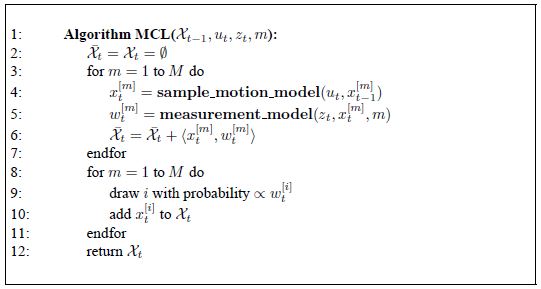
Monte Carlo Localization (MCL) is an advanced algorithm based on the Bayesian filter and the particle filter. Its primary purpose is to probabilistically estimate a robot’s pose within a predefined map. MCL consists of three main steps: prediction, which utilizes a motion model; measurement, which involves an observation model; and resampling. In our specific application, we use a motion model based on the wheel odometry of a non-holonomic mobile robot, and we gather sensor observations from point scans obtained through a 2D LiDAR.

MCL Algorithm (source: Probabilistic Robotics[1])
Motion Model
This model with regards to robot’s kinematics serves as state transition model, represented as the posterior $p(x_t | u_t, x_{t-1})$ according to motion control $u_t$. The state variable $x$ represents the robot’s pose, defined as ${x, y, \theta}$, which includes position and orientation based on the kinematics of a 2D mobile robot. The wheel odometry model predicts how the pose changes ($\Delta x, \Delta y, \Delta \theta$) in response to wheel movements.
- Defence against the irregularities
We utilized translation data from the odometer driver and orientation information from the IMU driver. Although the information is received periodically through a ROS2 node, there are occasional irregularities in the time interval. Applying defensive code for this when calculating the relative pose is a critical concern for several modules.
When representing the relative pose due to motion, as explained in Probabilistic Robotics[1], we decomposed $u_t$ into three motion parameters and applied noise to each of these parameters. 4 noise parameters related to translation and rotation are used to determine the variance of the error distribution.
Odometry performance profiling
We recognized the importance of conducting detailed performance profiling to evaluate the reliability of data obtained from odometry. As a result, we carried out experiments to compare the pose predictions from odometry with ground truth data obtained through motion capture. This approach involved analyzing the paths generated by motion capture and odometry when the robot returned to the same location after undergoing complex motion in a confined space. The results demonstrated that odometry performance closely matched ground truth data, thus establishing a solid foundation for having confidence in the fundamental performance of wheel odometry under normal conditions when addressing localization issues in the future.Importance of parameter tuning
In various real experiments conducted in specific environments, such as uphill terrain, I’ve noticed the significant influence of these noise parameters on the robot’s localization performance. Occasionally, these physical conditions introduce additional noise into odometry, which deviates from typical scenarios. Variations in the physical state and the reliability of driver-provided values can also lead to differences, even among robots of the same type. Furthermore, alterations in robot hardware can cause increased odometry noise due to mechanical characteristics. Therefore, it is vital to validate the fundamental performance of odometry and carry out precise parameter tuning customized for the particular robot in question.
Observation Model
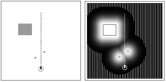
This model plays a important role in estimating the likelihood of different robot poses given sensor measurements. The model defines the sensor model, including details about sensor characteristics, such as noise, range, and field of view. It represents how well the predicted sensor readings (based on the particle’s pose) match the actual sensor measurements. The model can be represented as the conditional probability $p(z_t \mid x_t, m)$ of observing the actual sensor measurements $z_t$ given the particle’s pose $x_t$ in the map $m$. The probability is ideally the product of the individual measurement likelihoods, $\prod_{k=1}^K p(z_t^k \mid x_t, m)$.

Likelihood Field (source: Probabilistic Robotics[1])
For each particle’s pose, the expected sensor readings are calculated to determine what sensor data would be expected to receive if the robot were at that pose. Then, the particles are evaluated by comparing with the actual sensor measurements as the ground truth. The likelihood function is needed to quantify the similarity between them. We modeled the function based on our LiDAR’s characteristics modifying the probability distributions proposed in the book [1]. It gives the probability of observing the actual measurements given a particle’s pose. Further, it is also used in the resampling step to update particle weights and estimate the robot’s pose accurately in real time. I found that a well-defined and accurate observation model is critical for the success of MCL in robot localization tasks.
LiDAR performance profiling
We wanted to assess the performance limitations of LiDAR and determine the extent to which the characteristics of range, field of view, and noise align with the information provided in the datasheet. Additionally, we conducted LiDAR profiling due to the range quantization issue that arises when measuring distances up to the maximum range. In this phenomenon, when the robot approaches or moves away from a flat wall while looking at it vertically, the wall, which should be represented as a continuous straight line, appears to scatter into discrete points as if noise is introduced. This intermittently occurs from around a 10-meter point, becoming more pronounced from approximately 16 meters. To account for this uncertainty, we conducted these tests for various rotation frequencies to examine the distance-dependent noise characteristics of LiDAR measurements and incorporate such uncertainty into the sensor model.Likelihood Field Enhancement
To be added.
Resampling
When resampling, we use the likelihood, computed in the previous step to assign probabilities to each particle. States that generate sensor readings compatible with the actual measurements will have higher probabilities of being selected during resampling.
In the resampling process, it is essential to dynamically adjust the shape of the particle distribution or the number of particles at each step while accurately reflecting the uncertainty. However, this was not the case in the previous approach. To address this, we implemented the proposed KLD resampling as an Adaptive Particle Filter [3]. When observations are insufficient, we aimed for increased variance and a higher number of particles. Conversely, when observations are abundant, reducing uncertainty, we desired a narrower particle distribution with fewer particles for efficient computation.
- Particles exhibiting a line shape distribution
In the previous version of the MCL module, there was an issue where particles appeared in a discontinuous line shape rather than the typical continuous oval distribution. This problem arose due to the misconfiguration of the noise factor in the motion model, specifically, the translation-to-rotation noise, which was incorrectly set to 0. Consequently, during the resampling process, only particles aligned with the left and right walls and parallel to them would survive, while particles not aligned with the robot’s direction were entirely disregarded. By adjusting the value to an appropriate setting, we were able to achieve a normal particle distribution and experience the impact of noise parameter tuning.
Outcome
By testing in various environments and exploring artificial edge cases of sensor noise, we were able to confirm the performance advantage compared to the previous version. Through this process, we successfully applied the refactored outcome, achieving our goal of faithfully implementing the fundamentals of MCL while also resolving and validating the issues present in the previous version.
References
[1] Probabilistic Robotics [pdf]
[2] Particle Filter [pdf]
[3] KLD Sampling: Adaptive Particle Filter [pdf]
[4] Robust MCL for mobile robots [pdf]
[5] MCL with Mixture Proposal Distribution [pdf]
Yes! I finally stepped into the research on autonomous mobile robots that I had been longing for. To acquire the necessary knowledge in this field, I went through the process of reading numorous textbooks, lecture materials, and papers, as well as taking external courses, to thoroughly understand the content. Embarking on independent research was by no means easy. Furthermore, applying and adapting this knowledge to real-life situations and gaining insights required a lot of practice. Adapting to the environment of growth as a researcher, I progressed from MCL and forward planning tasks, following our team’s task rotation policy at the time, and embarked on the current Visual SLAM task.
